

Inflation does not always respond to cost and demand pressures in the same way. When shocks are small, the mapping from costs to prices is roughly proportional—double the shock, double the inflation response. But when the economy is hit by large shocks, this proportionality breaks down. As the recent surge and subsequent decline of global inflation showed, price growth can accelerate—or decelerate—by more than one-for-one relative to the size of the disturbance. Economists refer to this pattern as nonlinear inflation dynamics. In this post, I discuss what these nonlinearities mean, how they relate to the slope of the Phillips curve discussed in a companion post, and how firm-level data can help us understand the mechanisms behind them.
Evidence of Nonlinearities in the Data
The chart below illustrates nonlinear inflation dynamics taken from a recent working paper. It plots a measure of real cost changes for the Belgian manufacturing sector against producer price inflation (PPI) over the period 1999–2023.
The Nonlinear Relation Between Inflation Cost Shocks and Inflation
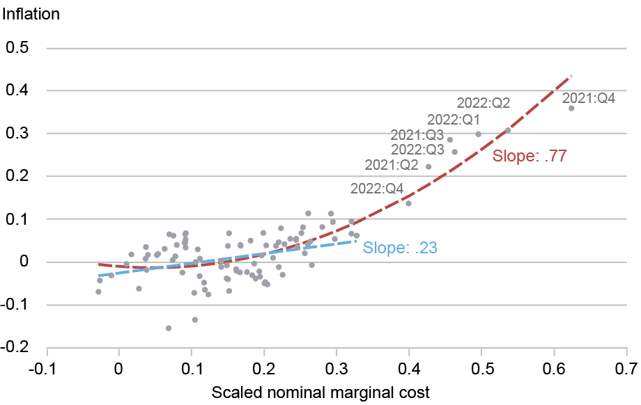
Notes: Each dot represents the joint realization of year-over-year change in a production-cost index (x-axis) against year-over-year PPI inflation (y-axis) for Belgian manufacturing in the same quarter. The data cover the period 2000:Q1 through 2023:Q4.
For small and medium-sized cost shocks, inflation rises roughly one-for-one with costs: the dots align along a straight line. When the economy is under stress, however, this proportionality breaks down. Once cost shocks exceed a threshold—around a 20 percent annual increase in our data—the slope steepens sharply. Double the size of the shock and inflation rises by much more than twofold. That is, inflation becomes more sensitive to shocks when disturbances are sufficiently large. This pattern is exactly what we observe in recent years, when the energy shocks and supply-chain disruptions associated with the COVID-19 pandemic and the war in Ukraine drove exceptionally large increases in producers’ costs.
The State-Dependent Nature of Pricing
Nonlinear inflation dynamics reflect the microeconomics of firms’ pricing decisions—and, in particular, the state-dependent way firms respond to shocks. Simply put, firms do not react uniformly: when shocks are small, many wait; when shocks are large, more firms adjust, and by larger amounts.
To see the intuition, consider a world where firms can adjust prices only at random and with a fixed probability—like in a lottery. In this world, the firms that reprice are not necessarily those facing the largest shocks (those whose prices deviate most from their optimal level). Yet when they do reprice, they update their prices to reflect current economic conditions. These ideas underlie the Calvo model, the workhorse model used in academic and policy analysis. In this framework, the average frequency of price changes does not vary with economic conditions, implying that inflation scales linearly with the size of the shock (a linear Phillips curve). Strict as they may seem, the assumptions behind the Calvo model—particularly the fixed probability of price adjustment—are remarkably consistent with the data in normal times.
Things look different when shocks are large. If adjusting prices is costly—because, for example, it involves updating menus or risks alienating customers—firms reprice only when the benefits outweigh those costs, much as a restaurant rewrites its menu only when prices are far out of date. When pressures are modest, few firms find it worthwhile; when shocks surge, many do. These shifts show up clearly in the data: large jumps in the average frequency of price changes occurred, more recently, during the recent pandemic inflation surge.
Such spikes are inconsistent with the Calvo model, but they are exactly what state-dependent pricing models—such as menu-cost models or models with information frictions—predict. These models capture the idea that when the economy is hit by large shocks, the entire price-setting process speeds up.
Three Facts About Pricing
Using detailed administrative data on thousands of Belgian manufacturing firms, we construct an empirical measure of each firm’s price gap—the percentage difference (in percentage terms) between the price it currently charges and the price it would set if it could adjust freely (its “desired price”). The larger the gap—whether positive or negative—the greater the changes in costs or competitive pressures the firm faces, and the further its current price drifts from the desired one. We thus provide a natural way to study how often and by how much firms adjust in response to shocks of different sizes.
Fact 1: Firms adjust more frequently when their prices drift far from optimal
The chart below shows the relationship between firms’ price gaps and the frequency of price adjustment. The blue line represents the probability density function of price gaps and the red line the fraction of firms that adjust their prices (y-axis) at each point of the price gap distribution. Firms in the tails—those with prices far above or below their desired price level—change prices much more often. The relationship is U-shaped: the further a firm’s price is from its target, the more likely it is to adjust. This is exactly what state-dependent pricing models predict. By contrast, in the Calvo model the probability of adjustment is unrelated to the price gap—its predicted curve would be flat.
The Probability of Price Adjustment Rises with the Size of the Price Gap
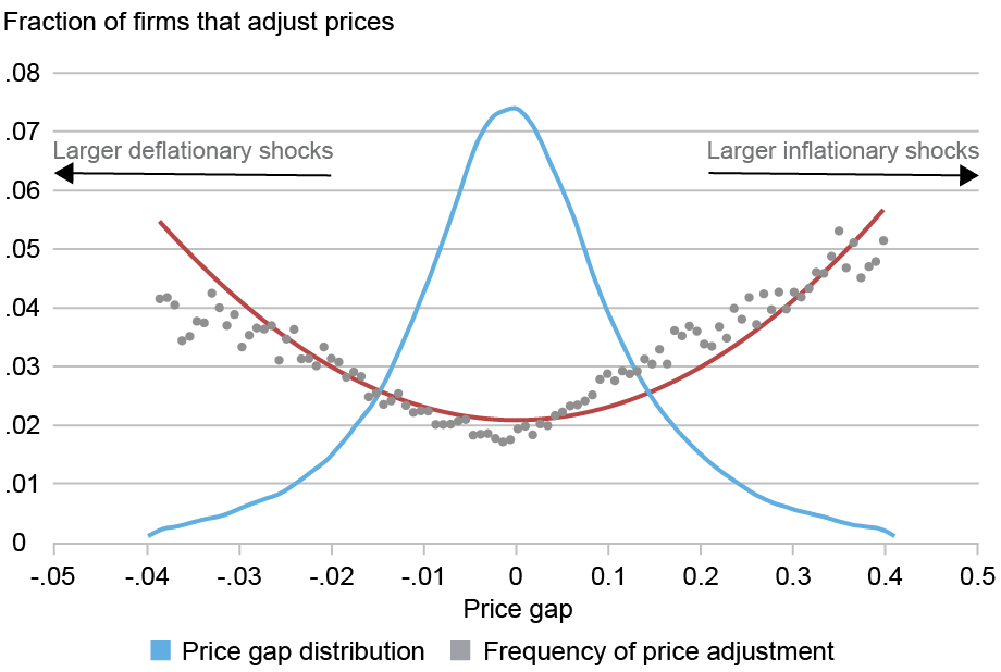
Notes: The blue line represents the probability density function of the distribution of price gaps; the red line shows the measured frequency of price adjustment along the price gap distribution.
Fact 2: Large aggregate shocks shift the entire distribution of price gaps, prompting more frequent price changes
The chart below shows how aggregate shocks reshape firms’ incentives to reprice. Before the pandemic, the distribution of price gaps was centered around zero (blue line). In 2022:Q2—the quarter with the largest jump in firms’ production costs—the entire curve shifts rightward (red dashed line) as producers grappled with surging energy prices and widespread supply chain disruptions, and, as predicted by state-dependent pricing, the share of firms changing prices nearly doubled, leading to a marked acceleration in inflation.
Large Aggregate Shocks Shift the Entire Distribution of Price Gaps, Prompting More Frequent Price Changes
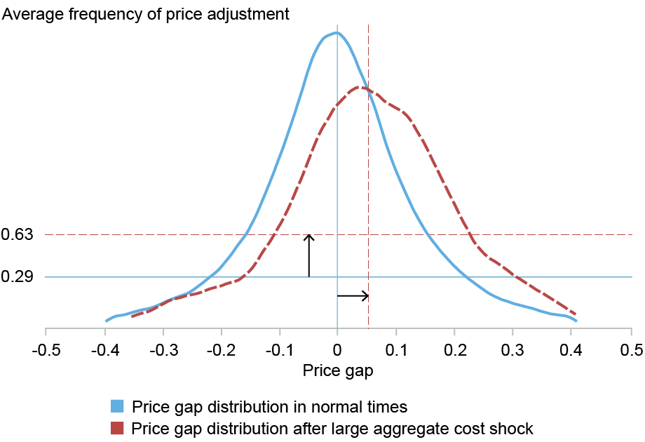
Notes: The blue curve is the pre-pandemic (1999–2019) density of price gaps; the red dashed curve is the 2022:Q2 density. Vertical lines mark the average gaps in the pre-pandemic period and in 2022:Q2. Horizontal lines show average adjustment probabilities in each period.
Fact 3: Inflation grows disproportionately larger when large shocks hit
In the chart below, we again group firms by the size of their price gap. Each dot represents the average price gap for a group of firms (x-axis) plotted against their average price change (y-axis). The red dashed line shows a nonlinear fit through this cloud of points.
Inflation Responds Nonlinearly with the Size of the Shocks to Firms’ Desired Prices
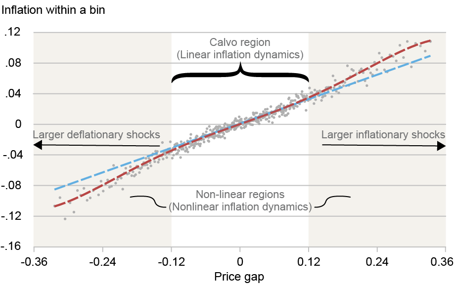
Notes: The blue dashed line represents a linear fit of price changes (inflation) on price gaps, estimated on the subsample of bins covering firms between the 25th and 75th percentiles of the price gap distribution, with the estimated slope reported in black. The red dashed line represents the fit of a third-order polynomial in price gaps, estimated using bins across the entire price gap distribution.
At any point along this curve, its slope measures how strongly cost shocks are passed through into prices—the steeper the slope, the stronger the pass-through, and the steeper the Phillips curve. This exercise reveals that the mapping between expected price changes and price gaps is not constant. In fact, we can identify two distinct regions.
The Calvo region. When price gaps are small (roughly +/- 10 percent), pricing behavior looks linear: adjustment frequencies are stable, pass-through is proportional, and the elasticity of price changes with respect to gaps matches the average adjustment frequency. This pattern helps explain why the Calvo model works well in low-inflation environments.
The nonlinear regions. At the tails of the price gap distribution, pricing becomes far more reactive. Firms hit by large shocks exhibit nearly double the usual pass-through due to the significant rise in the frequency of price adjustment. The behavior of these firms mirrors what happens to the broader economy during major disturbances—such as those triggered by the COVID-19 pandemic. During these episodes, the economy is pushed into regions where the slope of the Phillips curve rises, and inflation reacts much more strongly and quickly to cost pressures.
Recognizing when the economy shifts between these regimes is important for decision makers who rely on timely signals about changing inflation conditions. Accounting for these transitions is key to understanding how inflation builds and eventually unwinds.

Simone Lenzu is a financial research economist in the Federal Reserve Bank of New York’s Research and Statistics Group.
How to cite this post:
Simone Lenzu, “Does the Phillips Curve Steepen When Costs Surge?,” Federal Reserve Bank of New York Liberty Street Economics, February 5, 2026, https://doi.org/10.59576/lse.20260205
BibTeX: View |
Disclaimer
The views expressed in this post are those of the author(s) and do not necessarily reflect the position of the Federal Reserve Bank of New York or the Federal Reserve System. Any errors or omissions are the responsibility of the author(s).